!pip install pytorch_lightning
!pip install -U git+https://github.com/qubvel/segmentation_models.pytorch
!pip install watermarkIn this example, we will build an image segmentation model to segment the 3 different classes in the Oxford-IIIT Pet Segmentation Dataset.
We’ll use Segmentation Models PyTorch which was introduced in an earlier post on Surface Defect Segmentation, but in this post we focus on Torchmetrics, which is a new library that has many metrics for classification/segmentation in Pytorch. Torchmetrics
- Allows for easy computation over batches.
- Is rigorously tested.
- A standardized interface to increase reproduciblity.
- And much more…
Torchmetrics was already introduced for Pet Breed Classification, but in this post we’ll describe the mdmc_average parameter which is relevant for higher dimensional image data.
First we’ll install Torchmetrics with PyTorch Lightning below.
import os
import random
import collections
import numpy as np
import torch
import torchvision
import matplotlib.pyplot as plt
# for plotting
plt.rcParams["figure.figsize"] = (10.0, 8.0) # set default size of plots
plt.rcParams["font.size"] = 16
from pytorch_lightning import LightningModule, Trainer, seed_everything
import segmentation_models_pytorch as smp
import torchvision.transforms.functional as TF
from torch.utils.data import random_split
seed_everything(7)Global seed set to 77Exploratory Data Analysis
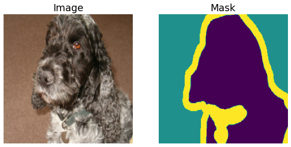
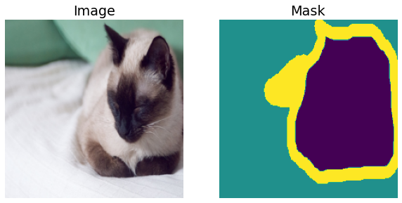
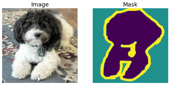
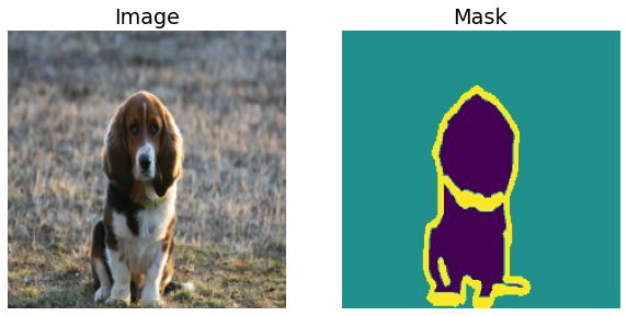
We’ll first look at some image/mask pairs in the dataset and basic dataset statistics. To do this, we’ll resize the images to a standard size of \(224 \times 224\).
def transforms(image,target):
image, target = TF.resize(image,(256,256)), TF.resize(target,(256,256))
image, target = TF.center_crop(image,224), TF.center_crop(target, 224)
# Shift the indicies so that they are from 0,...,num_classes-1
return TF.to_tensor(image), 255*TF.to_tensor(target) - 1# set download to False after the dataset is downloaded.
vis_dataset = torchvision.datasets.OxfordIIITPet(root="./data", split="trainval", target_types="segmentation",transforms=transforms,download=True)Downloading https://thor.robots.ox.ac.uk/~vgg/data/pets/images.tar.gz to data/oxford-iiit-pet/images.tar.gzExtracting data/oxford-iiit-pet/images.tar.gz to data/oxford-iiit-pet
Downloading https://thor.robots.ox.ac.uk/~vgg/data/pets/annotations.tar.gz to data/oxford-iiit-pet/annotations.tar.gzExtracting data/oxford-iiit-pet/annotations.tar.gz to data/oxford-iiit-petAs we shall see below, the segmentation masks have 3 labels (see the Cats and Dogs original paper):
- Pet Body
- Background
- Ambiguous region (between body and background)
for i in range(5):
sample_img, sample_msk = vis_dataset[random.choice(range(len(vis_dataset)))]
plt.subplot(1,2,1)
plt.title("Image")
plt.axis("off")
plt.imshow(sample_img.permute([1,2,0]))
plt.subplot(1,2,2)
plt.title("Mask")
plt.axis("off")
plt.imshow(sample_msk.permute([1,2,0]).squeeze())
plt.show()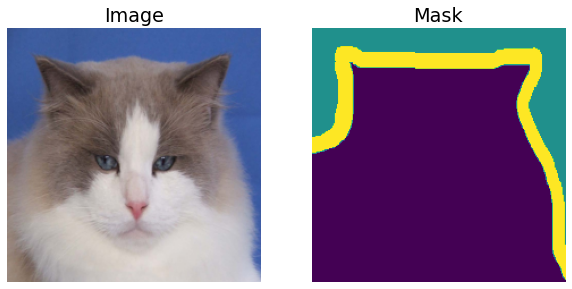
Now we’ll calculate the mask statistics.
# Use a dataloader to speed up the loading of masks.
vis_dataloader = torch.utils.data.DataLoader(vis_dataset, shuffle=False, batch_size=16, num_workers=os.cpu_count())
pixel_counts = collections.defaultdict(int)
for _, mask in vis_dataloader:
labels, counts = np.unique(mask.numpy(),return_counts=True)
labels = list(map(int, labels))
for label, count in zip(labels,counts):
pixel_counts[label] += count
# Work with normalized counts
pixel_counts = np.array(list(pixel_counts.values()))/sum(pixel_counts.values())As the figure below shows, our dataset is mildly imbalanced. Thus as mentioned in the Surface Defect Segmentation post, it makes sense to experiment with different loss functions offered by the segmentation models library.
fig, ax = plt.subplots(figsize=(8,5))
ax.barh(range(len(pixel_counts)), pixel_counts)
width=0.15
ind = np.arange(3)
ax.set_yticks(ind+width/2)
ax.set_yticklabels(["Body", "Background", "Border"], minor=False)
plt.xlabel("Number of pixels per class")
plt.title("Distribution of pixel labels")
plt.show()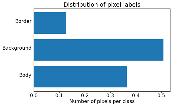
Training
Define data augmentations to use with the train dataset. More data augmentations are possible with the albumentations library.
def train_transforms(image,target):
# Only horizontal flips
if random.random() < 0.5:
image = TF.hflip(image)
target = TF.hflip(target)
image, target = TF.resize(image,(256,256)), TF.resize(target,(256,256))
image, target = TF.center_crop(image,224), TF.center_crop(target, 224)
# Shift the indicies so that they are from 0,...,num_classes-1
return TF.to_tensor(image), 255*TF.to_tensor(target) - 1def val_transforms(image,target):
image, target = TF.resize(image,(256,256)), TF.resize(target,(256,256))
image, target = TF.center_crop(image,224), TF.center_crop(target, 224)
# Shift the indicies so that they are from 0,...,num_classes-1
return TF.to_tensor(image), 255*TF.to_tensor(target) - 1# Set the download parameter to False after the datasets are downloaded.
train_dataset = torchvision.datasets.OxfordIIITPet(root="./data", split="trainval", target_types="segmentation",transforms=train_transforms,download=False)
val_dataset = torchvision.datasets.OxfordIIITPet(root="./data", split="test", target_types="segmentation",transforms=train_transforms,download=False)print('Length of train dataset: ', len(train_dataset))
print('Length of validation dataset: ', len(val_dataset))Length of train dataset: 3680
Length of validation dataset: 3669num_classes = 3
BATCH_SIZE = 16train_dataloader = torch.utils.data.DataLoader(train_dataset, shuffle=True, batch_size=BATCH_SIZE, num_workers=os.cpu_count())
val_dataloader = torch.utils.data.DataLoader(val_dataset, shuffle=False, batch_size=BATCH_SIZE, num_workers=os.cpu_count())Now we’ll subclass the LightningModule to create and train the model. The code below is similar to that in Pet Breed Classification and Surface Defect Segmentation, with the main difference being the metrics we define below.
We’ll use the Accuracy and F1Score with torchmetrics to measure the performance of our model. The main difference from the pet breed classification example (which describes the average parameter) is that now we have to use the mdmc_average parameter to reduce the extra image dimensions, \(H\) and \(W\). We shall use mdmc_average=global, which is described in greater detail below.
For a given batch of data of shape \([B, C,H,W]\), the option mdmc_average=global collapses the data into shape \([B\times H \times W, C]\) and then calculates the F1Score as for multiclass classifiers. The option mdmc_average=samplewise on the other hand calculates the F1score for each of the \(B\) samples and each of the \(C\) classes, and then averages over the sample and class dimensions (cf. F1Score). The logic is similar for other metrics like the Dice score for example. This will be elaborated in an upcoming post, giving comparisons with the metrics in segmentation models pytorch, and recommendations for practical usage.
import torch.nn as nn
from torchmetrics import MetricCollection, Accuracy, F1Score
from torch.nn import functional as F
class PetModel(LightningModule):
def __init__(self, arch, encoder_name, learning_rate, num_classes, loss="DiceLoss", **kwargs):
super().__init__()
self.save_hyperparameters()
self.example_input_array = torch.zeros((BATCH_SIZE, 3, 224,224))
# Setup the model.
self.model = smp.create_model(
arch, encoder_name=encoder_name, encoder_weights = "imagenet", in_channels=3, classes=num_classes, **kwargs
)
# Setup the losses.
if loss == "CrossEntropy":
self.loss = nn.CrossEntropyLoss()
else:
self.loss = smp.losses.DiceLoss(smp.losses.MULTICLASS_MODE, from_logits=True)
# Setup the metrics.
self.train_metrics = MetricCollection({"train_acc" : Accuracy(num_classes=num_classes, average="micro",mdmc_average="global"),
"train_f1" : F1Score(num_classes=num_classes,average="weighted",mdmc_average="global")})
self.val_metrics = MetricCollection({"val_acc" : Accuracy(num_classes=num_classes, average="micro",mdmc_average="global"),
"val_f1" : F1Score(num_classes=num_classes,average="weighted",mdmc_average="global")})
self.test_metrics = MetricCollection({"test_acc" : Accuracy(num_classes=num_classes, average="micro",mdmc_average="global"),
"test_f1" : F1Score(num_classes=num_classes,average="weighted",mdmc_average="global")})
def forward(self, x):
return self.model(x)
def training_step(self, batch, batch_idx):
images, targets = batch
#TODO: do this at dataset preparation.
targets = targets.squeeze().long()
logits_mask = self.forward(images)
loss = self.loss(logits_mask, targets)
preds = torch.softmax(logits_mask, dim=1)
self.train_metrics(preds, targets)
self.log("train_acc", self.train_metrics["train_acc"], prog_bar=True)
self.log("train_f1", self.train_metrics["train_f1"], prog_bar=True)
self.log("train_loss", loss, prog_bar=True)
return loss
def evaluate(self, batch, stage=None):
images, targets = batch
targets = targets.squeeze().long()
logits_mask = self.forward(images)
loss = self.loss(logits_mask, targets)
preds = torch.softmax(logits_mask, dim=1)
if stage == "val":
self.val_metrics(preds,targets)
self.log("val_acc", self.val_metrics["val_acc"], prog_bar=True)
self.log("val_f1", self.val_metrics["val_f1"], prog_bar=True)
self.log("val_loss", loss, prog_bar=True)
elif stage == "test":
self.test_metrics(preds,targets)
self.log("test_acc", self.test_metrics["test_acc"], prog_bar=True)
self.log("test_f1", self.test_metrics["test_f1"], prog_bar=True)
self.log("test_loss", loss, prog_bar=True)
def validation_step(self, batch, batch_idx):
return self.evaluate(batch, "val")
def test_step(self, batch, batch_idx):
return self.evaluate(batch, "test")
def configure_optimizers(self):
return torch.optim.Adam(params=self.parameters(), lr=self.hparams.learning_rate)We’ll start off with the UNET architecture using a resnet34 backbone. Other options include using the DeepLabV3 architecture and the RegNetX backbone for slightly higher accuracy.
model = PetModel("UNET", "resnet34", 1e-3, num_classes, loss="CrossEntropy")Downloading: "https://download.pytorch.org/models/resnet34-333f7ec4.pth" to /root/.cache/torch/hub/checkpoints/resnet34-333f7ec4.pthWe’ll log metrics to TensorBoard using the TensorBoardLogger, and save the best model, measured using F1Score, with the ModelCheckpoint. Note that we use the F1Score instead of Accuracy because of the mild class imbalance.
from pytorch_lightning.loggers import TensorBoardLogger
from pytorch_lightning.callbacks import ModelCheckpoint
name = "oxfordpet" + "_" + model.hparams.arch + "_" + model.hparams.encoder_name + "_" + model.hparams.loss
logger = TensorBoardLogger(save_dir="lightning_logs",
name=name,
log_graph=True,
default_hp_metric=False)
callbacks = [ModelCheckpoint(monitor="val_f1",save_top_k=1, mode="max") ]from itertools import islice
def show_predictions_from_batch(model, dataloader, batch_num=0, limit = None):
"""
Method to visualize model predictions from batch batch_num.
Show a maximum of limit images.
"""
batch = next(islice(iter(dataloader), batch_num, None), None) # Selects the nth item from dataloader, returning None if not possible.
images, masks = batch
with torch.no_grad():
model.eval()
logits = model(images)
pr_masks = torch.argmax(logits,dim=1)
for i, (image, gt_mask, pr_mask) in enumerate(zip(images, masks, pr_masks)):
if limit and i == limit:
break
fig = plt.figure(figsize=(15,4))
ax = fig.add_subplot(1,3,1)
ax.imshow(image.squeeze().permute([1,2,0]))
ax.set_title("Image")
ax.axis("off")
ax = fig.add_subplot(1,3,2)
ax.imshow(gt_mask.squeeze())
ax.set_title("Ground truth")
ax.axis("off")
ax = fig.add_subplot(1,3,3)
ax.imshow(pr_mask.squeeze())
ax.set_title("Predicted mask")
ax.axis("off")Sanity check the model by showing its predictions.
show_predictions_from_batch(model, val_dataloader, batch_num=3, limit=1)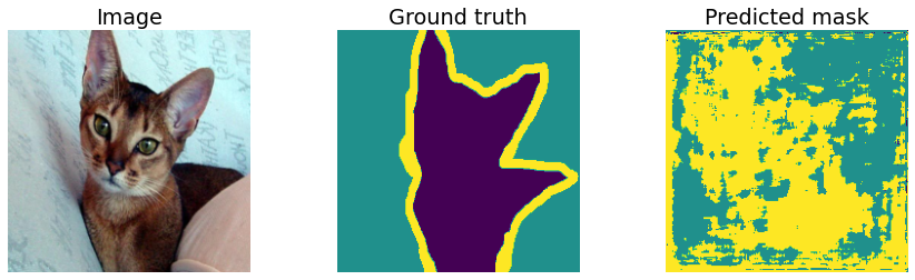
Visualize training progress in TesnorBoard.